Mathematical Principle of VAE

---

Introduction

Within just three years, along with GAN, Variational Auto-encoder (VAE) became the most popular method of unsupervised learning of complicate probability density. This is because VAE is built upon standard approximation units, i.e. neural networks and thus can be trained using stochastic gradient descent. This work will focus on the philosophical and intuitive interpretations and the related mathematical principles.

Inherited from the learning and predicting mechanism of traditional auto-encode, VAE encodes and decodes between measurable functions. Like GAN, the most important idea is based on a stunning mathematical fact: for a target probability distribution T, given any distribution S, there exists a differentiable measurable function that maps S to another probability distribution A such that A approximates T with any precision.

In measure theory, measurable function is the mapping from the measurable space of the real world to that of math. Naturally, the latter one is chosen to be Euclidean space with Borel σ-field. Following graphical models, in VAE, we expect to generate samples from some latent variable. For example, suppose we want to generate manuscript 0-9. There are numerous contributing factors that influence the style of these numbers, such as the strike, the angle of the pen, the writing habit of the writer, the weather (the weather will affect the mood thus affect the writing style; according to butterfly effect, even the subtle change of the initial condition will eventually influence the consequence). One straightforward way is to enumerate the probability distribution of all these latent factors. However, this is impractical because there are just too many of them and we don’t want to handcraft these factors. VAE circumvents this intractability by modelling the distribution of latent measurable variables with a joint Gaussian distribution (this latent measurable function maps all these latent factors into Euclidean space). Then, the problem is reduce to learning a mapping from a latent measurable function (random variable) to samples to be generated. This process is called decoding. One could imagine how complicate this mapping would be. Then, we must resort to deep learning with its strong approximating ability.

Derivation

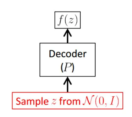
As discussed above, we want to obtain a generative model shown below.

where z is the latent random variable(latent measurable function). z will be sent to a decoder and thus transformed into f(z) such that f(z) resembles as much as possible to the genuine one with diversity.

How could such a decoder be learned?

We will start from the objective. Suppose we have the genuine samples S={x(i),i=1,...,m}, for instance, back to our previous example, we have samples of manuscripts 0-9. More similar and diverse samples are expected to be generated. Therefore, the learnable parameters Θ are learned using maximum likelihood. Formally, we have

Without loss of generality, we only consider a single sample x for simplicity. Note that the above objective is a function of x only. We should make out of the latent random variable z.

where q(z|x) is a certain conditional probability distribution of z given x.

But why do we choose such a conditional distribution rather than q(z) or p(z|x)?

This is because there are too many q(z) to choose from. Instead, we are more curious about those z with much likelihood of generating x. As for p(z|x), p(⋅) can be deemed as a real but unknown probability distribution that only God knows. What we want to do is to approximate p(⋅) with q(⋅). q(⋅) can be regarded as a certain approximating distribution.

Continue with the derivation,

By Bayesian formula, the first term

Consequently, we obtain the core equality of VAE,

Now we start to introduce assumptions

Likewise, q(z|x) and p(x|z) are modelled by Gaussian distributions,

Then, it is quite obvious that we resort to neural networks to learn these four mappings. Unfortunately, DKL(q(z|x)||p(z|x)) is still intractable (the normalizer is a intractable multi-integral). We have to step back for sub-optimization,

We maximize the lower bound of the log likelihood.

Plugging the assumption into the lower bound and setting Λ(z) to be I, irrelevant of z for simplicity, yields

Maximizing the lower bound is equivalent to minimizing the quantity

where Θ is the set of the learnable parameters of the four mappings.

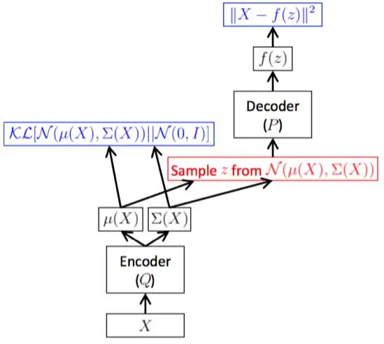
Consequently, we obtain the whole learning framework as shown below.

To summarize, the whole training framework is encoding and decoding the sample x. q encodes x into the latent variable z, and p decodes z back to f(z) with the reconstruction error minimized. The training objective is to learn mappings of the encoder and the decoder. Therefore, we are actually conducting variational inference of Q, as the name VAE implies.

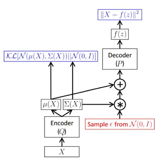
However, in practice, back propagation is unable to be performed during the phase from the decoder to “μ(x) and Σ(x)”. Indeed, the above epigraph is just for intuitive understanding. As shown below, practically, we resort to reparameterization to make it possible.

The reparameterization is not so mysterious as it sounds. It is simply based on a simple mathematical fact:
Suppose z∼(μ,Σ), then the random variable z can be written as

where ϵ∼(0,I).

By this trick, we can circumvent this intractability.

Discussion

A. Any probability distribution can be exploited as the distribution of the latent random variable. Why Gaussian necessarily?

The answer may lie in two aspects. On one hand, modelling Gaussian results in computational tractability, thus we can obtain some analytical solutions. On the other, more importantly, it may be due to the following mathematical fact,

The solution to this optimization problem is

This indicates given the mean and the variance, the one with highest information entropy is Gaussian distribution.

B. Despite that we simply maximize the lower bound, with some designed network of sufficient capability, the objective logp(x)−DKL(q(z|x)||p(z|x)) is actually being maximized, which means the log likelihood is maximized (our ultimate objective) on one hand and on the other, the K-L divergence between q and p is minimized. If the K-L divengence is perfectly minimized, the intractable p(z|x) is made tractable by the approximation q(z|x).

C. K-L Divergence between Gaussians

Given two pdf p1=(μ1,Σ1) and p2=(μ2,Σ2), the divergence between them is

Reference

Tutorial on Variational Autoencoders. Carl Doersch. arXiv:1606.05908, 2016.